Exploring Numeric and Pygame

While I am typing this article in `vim', my GNU/Linux box is playing an old Malayalam movie song. The amazing thing is that what the brain perceives as `music' is nothing but a gigantic sequence of numbers being processed and converted to electrical signals by some intricate hardware and software on the computer. A number of libraries are available on the GNU/Linux platform for performing sophisticated mathematical computations on large datasets. Of particular interest to me (and I hope, all fellow Python fans) is the `Numeric' module which brings in high-speed matrix processing to the relatively `slow' world of Python. This article provides an introduction to Numeric by using it in conjunction with two other libraries - `Pygame' and `Matplotlib'. Pygame is a graphics library built on top of SDL (Simple DirectMedia Layer) and Matplotlib is a sophisticated 2D plotting package.

Getting started

The `Numeric' module provides a `multidimensional array' datatype and a set of fast operations capable of acting on the entire array (or a subset). Because the basic operations are defined very carefully, it is possible to express almost any complex matrix manipulation as a combination of a few of the primitive operations. Let's try out an experiment at the Python prompt:


>>> from Numeric import *
>>> a = array([1,2,3])
>>> print a + 1
[2 3 4]
>>> print a * a
[1 4 9]

There is one very important point to be noted in this example - that the array constructed as a result of calling the function `array' is not in any way similar to a Python list. Had that been the case, we would not have been able to add 1 to it. We also note that the operation of adding 1 to the array resulted in the values of all the elements getting changed and the operation of multiplying the array by itself resulted in an elementwise multiplication.

A few definitions

A Numeric multiarray (we will call it just `array') has a `rank' which is the number of dimensions or `axes' it has. For example, the rank of the following array is 1:


a = array([1,2,3])

The `length' of the array along this dimension is 3. The function `rank' returns the rank of the array which it gets as its argument.

The `shape' of an array is the set which defines the length of the array across each of its dimensions.


>>>
>>> a = array(([1,2,3],[4,5,6]))
>>> print a
[[1 2 3]
 [4 5 6]]
>>> a.shape
(2,3)
>>>

The shape of the array is (2,3) - ie, it contains two rows and three columns.

Reshaping Arrays

Let's start with the following array:


>>> a = arange(0,6)
>>> print a
[0 1 2 3 4 5]

We can now `reshape' it into a 2x3 matrix:


>>> b = reshape(a, (2, 3))
>>> print b
[[0 1 2]
 [3 4 5]])
>>> b[0] = 8
>>> print b
[[8 8 8]
 [3 4 5]])
>>> print a
[8 8 8 3 4 5]
>>> a.shape = (3, 2)
>>> print a
[[8 8]
 [8 3]
 [4 5]])
>>>

As long as the total number of elements does not change, it is possible to reshape the array in whatever way we like. In the above example, we first reshaped a 6 element one-dimensional array into a two-row and three-column array. Assigning a value to b[0] resulted in all the elements of that row getting changed to 8. We note that the array returned by `reshape' is not a copy of the original - it is just another `view' into the very same array. This explains the fact that changing `b' resulted in `a' also getting changed. Finally, the shape of an array is just one of its attributes, it can be modified by simply assigning a new tuple.

Zero's, one's and Random Arrays

Say you wish to create a 3x3 array of random integers in the range 0 to 20 (both inclusive):


>>> from RandomArray import *
>>> a = random_integers(20, 0, (3,3))
>>> print a
[[10 4 9]
 [12 6 20]
 [20 9 17]])
>>>

The functions `zeros' and `ones' are useful for creating arrays of identical values:


>>> print zeros((3,3)) - 5
[[-5 -5 -5]
 [-5 -5 -5]
 [-5 -5 -5]]
>>>

Plotting a sine wave

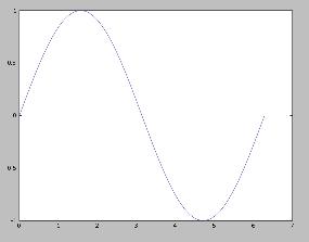
Let's now use the powerful `matplotlib' package to do some simple visualizations. Listing 1 shows a Python script which when executed displays the plot shown in Figure 1. The `arange' function creates an array of numbers from 0 to 6.28 in steps of 0.01. Applying the`sin' function on this array results in another array each element of which is the sin of the corresponding element in the original array. The `plot' function simply generates a 2D x-y plot.

Fourier Magic!

We encounter `signals' everywhere. The PC speaker generates sound by converting electrical signals to vibrations. We see the objects around us because these objects bounce back light signals to our eyes. Our TV and radio receive electromagnetic signals; we are literally immersed in a `sea of signals'. Analysis of signals is therefore of central importance to most branches of science and engineering.

Jean Baptiste Joseph Fourier, the 18th century French mathematician and revolutionary had an amazing insight that complex time varying signals can be expressed as a combination of sin/cos curves of varying frequency and amplitude. The mathematical techniques which he had developed based on this insight now find application in disciplines as diverse as neurophysiology and digital communication. Let's try to visualize a bit of Fourier's math using Numeric and Matplotlib!

Instead of plotting the equation


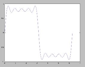
y = sin(x)

we will now combine a few sine wave's together and plot the resulting signal:


y = sin(x) + (1/3)*sin(3*x) + (1/5)*sin(5*x) + 
    (1/7)*sin(7*x) + (1/9)*sin(9*x)

Listing 2 shows a Python script which generates the plot shown in Figure 2; we note that the graph has become more complex. What if we keep on adding more sines (by changing `range(1,10,2)' to say `range(1,100,2)' in the program)? Our graph starts looking more and more like a square wave!

Graphics with Pygame

As the name suggests, Pygame is a Python framework for writing games. Combined with Numeric, it can be used for doing elementary image processing. My objective behind introducing Pygame is to demonstrate the utility of some of the fast matrix manipulation mechanisms offered by Numeric in a practical context.

Our first pygame program, shown in Listing 3 opens a window and displays the JPG image shown in Figure 3. You should run it by invoking


from listing3 import *

at the Python interpreter prompt.

The program starts off by invoking pygame.init to perform some initialization. A `surface' is an object on which you can perform graphics operations - the pygame.image.load function returns a surface which has an image mapped onto it. The pygame.surfarray.array3d function accepts a surface and returns a 3D array which contains the R,G,B values of each pixel of the image. In this case, the image has a size of 370x158 - imgarray[0] to imgarray[369] represent 1 pixel-wide vertical slices of the image from left to right. The pygame.display.set_mode function returns a special surface - special in the sense whatever is mapped on to this surface will appear on the screen. The first argument to this function is the (width,height) of the surface, the second argument is a flag and the third argument represents `depth' (bits per pixel). The blit_array function copies the contents of imgarray to `screen' and the pygame.display.flip function updates the contents of the display.

Slicing arrays

Before we do a few simple image manipulations, let us examine the very powerful (and sometimes confusing) slicing mechanism provided by Numeric.

We start with a one dimensional array:


>>>
>>> a = arange(10)
>>> print a[1:8:2]
[1 3 5 7]
>>> print a[8:1:-2]
[8 6 4 2]
>>> print a[7:]
[7 8 9]
>>> print a[:1:-2]
[9 7 5 3]
>>> print a[::-1]
[9 8 7 6 5 4 3 2 1 0]
>>> print a[::2]
[0 2 4 6 8]
>>>

Seems to be OK so far. The basic slice notation is:


array[start:end:step]

If step is +1 and start is lesser than end, this gives us all elements from index `start' to `end'-1 in increments of `step'. If step is -1 and start is greater than end, we get all elements from start to end+1. Either some or all these parameters can be missing, as demonstrated by some of the above examples. Say `start' is missing and step is negative - in this case, the start of the slice is assumed to be at the end of the array. Note that modifying the slice will result in the original array also getting modified.

Slicing is a bit more tricky when applied on multidimensional arrays:


>>>
>>> a = reshape(arange(9), (3,3))
>>> print a
[[0 1 2]
 [3 4 5]
 [6 7 8]]
>>> print a[0:2]
[[0 1 2]
 [3 4 5]]
>>> print a[0:2, 1:]
[[1 2]
 [4 5]]
>>> print a[:, -1]
[2 5 8]
>>> b = array(a)
>>> b[:, -1] = 10
>>> print b
[[0 1 10]
 [3 4 10]
 [6 7 10]]
>>> print b[:,::-1]
[[10 1 0]
 [10 4 3]
 [10 7 6]]
>>>

The expression a[0:2] gives us a slice of the 3x3 array composed of row numbers 0 and 1 and all the columns whereas writing a[0:2, 1:] yields a slice containing only elements from column numbers 1 and 2. The next expression, a[:, -1], takes the element in the last column from each row and returns a 1 dimensional array. Note that assigning to this slice will result in all the last column elements of the array changing.

Manipulating the image

Let's go back to the program which displayed a JPG file in a window. Each pixel is represented by a three element array containing the red, green and blue colour components - each row of `imgarray' contains 158 such three element arrays, the row as a whole representing a single bit wide vertical slice of the image. Just to make sure that we get the coordinate math correct, let's put a black vertical line at the center of the image:


>>>
>>> from listing3 import *
>>> imgarray[185] = [0, 0, 0]
>>> surfarray.blit_array(screen, imgarray)
>>> pygame.display.flip()
>>>

Let's try to flip the image vertically (Figure 4):


>>> surfarray.blit_array(screen, imgarray[:,::-1])
>>> pygame.display.flip()

What about a scaling-down operation? We simply choose alternate rows and columns from the original array by slicing both the dimensions with a step of two.


>>> s = imgarray[::2, ::2]
>>> screen = pygame.display.set_mode(s.shape[:2], 0, 24)
>>> surfarray.blit_array(screen, s)
>>> pygame.display.flip()

Finally, let's try to make the red component of each pixel equal to zero. This is simply a matter of identifying the proper integer slice and setting it equal to zero:


>>> imgarray[:,:,0] = 0

Interested readers should first construct a small 3D array and play with it a bit to understand what is really happening here.